Distance Decay of Magnetic Fields

To give a rough idea, if we compare the magnetizing force to a large magnet, the rate of distance-dependent decay depends on its length (the length of the magnetic moment).

If the magnetic moment is long, the decay with distance is gradual; if it is short, the decay is rapid.

A magnetic moment consists of two magnetic charge surfaces—the north pole and the south pole (which have a certain thickness).

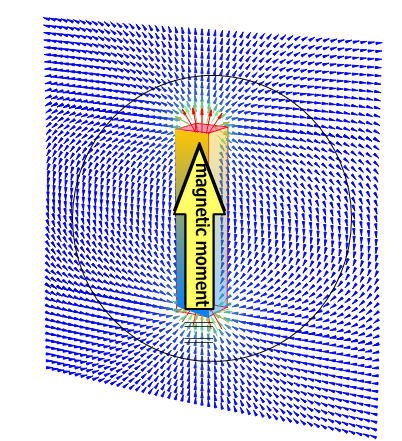
When represented by a single magnetic moment:
When the magnetic moment is aligned with the central axis, the magnetic field is weak except in the vicinity of the magnetic poles.
The sphere represents the Earth.

Of course, these are all just conceptual examples; Qm calculates a thick, three-dimensional coil using (discretized) three-dimensional currents.

If we express the above quantitatively as a mathematical equation,

The distance-dependent attenuation of electric and magnetic fields depends heavily on the shape of the source.

(1) As is well known from Coulomb’s law, the force from a point source is proportional to the inverse square of the distance.

\[H=C\dfrac{m}{r^2}\]
\(H:Magnetic Field　m:Magnetic Charge　r:Distance　C:const.\)

(2) For an infinitely long line source, the current is inversely proportional to distance, as shown by Ampère’s law.

\[H=C\dfrac{ρ}{r}\]
ρ:Lines-of-magntic-charge density

Ampère’s law, which pertains to electric current, is as follows.
\[H=\dfrac{I}{2\pi r}\]
I:current

（3）If the plate were infinitely large, there would be no distance attenuation.
\[H=Cσ\]
σ:Surface magnetic charge density

（4）For a line source of finite length, Biot-Savart’s law applies, and because the angle at which the source is viewed is taken into account, the result lies between (1) and (2).

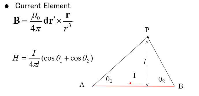
Even with complex coil winding configurations, everything can be broken down into current elements for calculation.

（5）This takes the form of an integral, with the curved surface S as the source. When the surface magnetic charge density is constant, it is proportional to the solid angle Ω between (2) and (3).

\[H=CΩ\]

\[Ω=\iint_s \dfrac{dS(r ,n)}{r^3}dr\]

Note that while the current relationships for Qm can be calculated as an application of Equation (4), for general ferromagnets, we use the analytical solution in Equation (5) (a theoretical solution, not a numerical solution obtained by dividing the problem into small segments).

All of these derive from conservation laws in three-dimensional space and are purely geometric (mathematical) in nature.