
What is electromagnetic field analysis software?
We provide various topics about electromagnetic field analysis, which is our specialty as a consultant.
目次
- 1 Approach to electromagnetic field analysis
- 2 Dimensions of the simulation model
- 3 Types of electromagnetic field analysis methods
- 4 Extra: The ultimate goal of technology?… Controllability and usefulness
Approach to electromagnetic field analysis
First of all,
From now on, I would like to provide various topics, starting with approaches to electromagnetic field analysis, but I think that those who come to this page are interested in electromagnetic field analysis for some reason or are planning to analyze electromagnetic fields in the future. If you are already doing electromagnetic field analysis, it may be a good idea to take a peek.
Why is electromagnetic field analysis necessary?
In a nutshell, electromagnetic field analysis does not mean that all current analysis methods and software can handle electromagnetic phenomena in a unified manner, and it is common to divide them into electric field analysis, magnetic field analysis, and electromagnetic wave analysis according to physical phenomena. Are. (Actually, it’s more finely divided.) In the future, software that can handle everything uniformly may be created, but it is doubtful that it will be possible even in 20 years because it is still a field that requires computer power. However, even if you cannot handle all electromagnetic phenomena in general, it is quite useful to analyze only the phenomena of particular interest in detail and accurately.
At the time of writing this article, it is as of 2002, but it is still not possible as of 2021. Theory and software technology rather than computer power are less advanced in this area, and very little has been done. I also wrote about “multiphysics” in the second part, but it is not very good. Even in modern times, little has changed.
My personal impression is that I have stepped back. This may also be due to the decline of manufacturing in Japan and other developed countries. It is not that cheap or bad, bad money drives out good money, but with the exception of some things, it is probably because they have come to demand cheapness rather than performance. Without even simulating it, if you imitate and use manufacturing equipment that has worked well so far, you can make most of it and ask for more. Is that enough financially? It may be, but if something big goes wrong, you won’t be able to deal with it. In addition, new technologies that will change the world and, for example, cause breakthroughs will not be born. Simulation is necessary to know what is happening, how to solve problems, to know the essence of things, to verify them, and to find new ways.
Whether or not the current problem can be solved depends on whether it is a problem that cannot be calculated unless all electromagnetic field phenomena can be handled in a unified manner, whether it can be calculated separately into electric field analysis, magnetic field analysis, or electromagnetic wave analysis, or whether it can be calculated more limitedly, as I will explain later. Roughly speaking, there are trade-offs between the many dimensions in space-time, the complexity of the model shape, and the complexity of physical properties. Here, as for the complexity of physical properties, whether it is a dielectric, a conductor, a magnetic material, a semiconductor, etc. … There are other classifications, such as nonlinearity and anisotropy.
For example, if we seriously model familiar magnetic phenomena, we will immediately take into account anisotropic hysteresis in 3D magnetic field analysis, and add the movement of magnetic materials and conductors and eddy currents, which is a very difficult analysis. Furthermore, when considering the displacement current involving dielectrics at the same time, it is necessary to perform coupled calculations of the dynamic magnetic field and the dynamic electric field, and as far as I know, there is currently no general-purpose software that can handle all of these at the same time. (Here, when I say “three-dimensional/general-purpose”, I am referring to software that can be calculated with arbitrary shapes, not software that is dedicated to motors or transformers.) )

Therefore, it is necessary to first clarify what to expect from electromagnetic field analysis and to define the requirements for the problem to be solved. After that, you will have to reconcile what you want with the limitations of the current analysis method and software. Of course, if you use multiple analysis methods and software, the range of defense will be wider. Depending on the combination, you may be able to solve quite complex problems. However, it requires a lot of experience, knowledge, a lot of effort and resources. On the other hand, if you accurately grasp the phenomenon that should be a problem and limit the model, you can find a solution accurately in a short time. Whichever approach you take, the craftsmanship element will remain quite strong. It is no exaggeration to say that this is the reason for the existence of our solver development manufacturer. Even if AI evolves, it cannot be trained without a huge amount of verified data.
Can you really solve the problems you are currently facing? Will you be satisfied with the solution?) First you need to know. In some cases, experimental/actual measurement may be a better choice than electromagnetic field analysis.
I wrote a lot of negative things, but I wrote them here because there are many people who have no prior knowledge and are doing or are doing electromagnetic field analysis. This corner was built in the hope that it would be of help to such people.
Electromagnetic field analysis that requires accuracy
Since the values of electric and magnetic fields are easier to measure directly than other analyses (because they are originally electrical signals…), the accuracy of the analysis is often strictly required. In addition, as a result of electromagnetic field analysis, secondary results such as stress and torque are often obtained based on the electric field and magnetic field obtained directly, so the electric field and magnetic field, which are the primary calculation results, must be obtained quite accurately.
For example, the stress caused by the magnetic field is proportional to the square of the magnetic field, and the torque is obtained by the difference, so the significant figure may be extremely small. Even if the error in magnetic flux density is 5%, the error in force and torque can be 100%. Recently, there is also a so-called inverse analysis (sensitivity analysis) in which the physical property value (conductivity from eddy current, etc.) is obtained from the measured value of the magnetic field. Even in such cases, the physical properties are determined from a slight change in the magnetic field, and considerable accuracy is required for analysis.
Also, as a background, many electromagnetic phenomena can be calculated analytically in real laboratory models, so the calculation error may be only the rounding error of the computer. In other words, as long as you do the calculations well (assuming that there is no confusion of physical phenomena), it is a natural world. This area is also slightly different from other CAE fields.
Example of a large error when converted to force
The magnetic field stress is proportional to the square of the magnetic field, and the resultant force is the difference. In other words, when stress is calculated from the result of the magnetic flux density on one surface, the significant figure is extremely small. Maxwell’s stress is
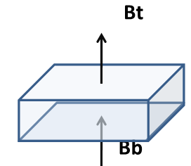
\(\mathbf{F} = \mu_r \mathbf{H (H・n)} – \cfrac{1}{2}\mu_r \mathbf{H^2}・\mathbf{n} \)
Top Field: \(\mathbf{B_t} = 100±5\) , Top stress: \(\mathbf{F_t} = c* (10000 ± 707.106)\)
Lower field: \(\mathbf{B_b} = 105±5\), Lower stress: \(\mathbf{F_b} = c*(11025 ± 742.462)\)
Resultant:\(\mathbf{F_b}-\mathbf{F_t}\)= c(11025 – 10000) ± \(\sqrt{742.462^2 + 707.106^2}\)
= c(1025 ± 1025.304)
Even if the error of the magnetic flux density is 5%, the error is 100% when converted into force.
Understanding the phenomenon to be analyzed
Therefore, it is important to understand the phenomenon to be analyzed and determine where the compromise can be made in the classification of magnetic field analysis described below. The right choice for your analysis purpose is the key to success. Please refer to the classifications in the next chapter and beyond, and use them as clues to solving your own problems.
Dimensions of the simulation model
Partitioning by geometry
The dimension or coordinate system of the space to be analyzed
- Zero-dimensional analysis: Spatial expansion is not considered. The so-called lumped constant system. It is often said that it is a one-point model.
- One-dimensional analysis: Problems solved as spherical symmetry
- Two-dimensional analysis: Problems solved as orthogonal systems ((x, y): infinite length in the z direction) or cylindrical systems (r, z)
- 3D analysis: Problems solved as orthogonal systems (x, y, z), polar coordinate systems (r, θ, z), or natural coordinate systems
The higher the dimensional level, the more accurate it is possible to analyze various effects and phenomena (three-dimensional rather than two-dimensional, three-dimensional dynamic analysis rather than three-dimensional static analysis, nonlinear analysis rather than linear analysis), but the number of variables handled increases exponentially, so it is necessary to select a model so that the accuracy of the solution of the problem of interest can be obtained.
A common approach is to take into account the space-time symmetry of the problem to be solved and reduce the dimensionality to make the problem easier to solve. For example, a problem in which the change in the electromagnetic field in the height (z) direction is small is solved as a two-dimensional (x,y) electromagnetic field analysis problem.
However, it should be noted that it is generally thought that a smaller dimension is easier to solve because of the smaller number of variables, but since the electromagnetic field problem is originally a three-dimensional (actually quaternary) problem, the reduction of the dimension may lead to cryptic terms, which may complicate the problem.

Zero-dimensional analysis (concentrated constant system) is sometimes used as an adjunct to the main analysis. In magnetic field analysis, external load circuits, power supply circuits, and current circuits fall under this category. Accumulated constants include the inductance of the coil as a circuit element, the capacitance of the capacitor, and the resistance value. In addition, if the response characteristics of high-dimensional analysis can be reduced as a zero-dimensional analysis problem by combining transfer functions and equations of state as dynamic calculation results, the range of applications and applications will expand.
* As an example of a game, attack power, defense power, … For example, those that are represented by multiple parameter sets are typical lumped constant system (0 dimensional) models. No matter how 3D the graphics are, it is common for the game parameters to have 0 dimensions. In this case, the same thing in the game breaks the pattern. However, in reality, no two things break in the same way.
Partitioning by time dependence
Electrostatic and magnetic field analysis without considering static analysis time terms. Even if the model moves, a static analysis is sufficient if the time-dependent terms listed in the dynamic analysis of the phenomenon of interest are negligible.
Example Stepper motor: Even if it is a moving object, the moment / moment can be calculated as if it were a photograph.- This analysis takes into account the dynamic analysis
time term. When we think of dynamic analysis, we tend to imagine that the model will move, but in reality, this is not the case, and the determining factor is whether the time-dependent term has a significant impact on the analysis results.
(1) Dynamic analysis in a narrow sense that focuses only on the movement of electromagnetic fields such as eddy current, back electromotive force, displacement current, and dynamic current (electric field analysis) when
the model does not move, and (2) Dynamic analysis in a broad sense that includes the movement and deformation of the model and changes in physical properties (due to the influence of temperature, force,
etc.) of the model that moves or deforms
.
In addition, there are stationary and non-stationary time-dependent terms. These also exist at the levels (1) and (2) above.
(A) Transient analysis, also called transient analysis
. It is an analysis that simulates transient or random phenomena over time. In most cases, there are analysis scenarios. For example, starting and stopping electromagnetic devices. Of course, even if there is no moving object, it also includes analyzing the change in the field when the power is turned on and disconnected. There are two types of transient time term analysis: explicit and implicit, which we will discuss in more detail later.
(B) Steady-state analysisA
phenomenon that repeats at a constant period. The phenomenon of the so-called “steady state” is analyzed, and there is a “equilibrium state” that is very similar to the “steady state”. In the “equilibrium state“, the actors are replaced even if there is no change in the object and the field (a certain balance is maintained with respect to time t in the macro sense). This is sometimes called a “steady state”, but in electromagnetic field analysis, solving the “equilibrium state” is not a steady state analysis, but it is classified as a static analysis. (Example: Direct current, which is generally handled in static magnetic field analysis, has a constant current flowing, but individual electrons do not stop.) In other words, in a steady-state analysis, it is an analysis that finds a field that changes periodically with respect to time t. - Magnetohydrodynamic analysis is a special type of “1. Dynamic analysis
(2) Moving or deforming the model” classified above, but it is further divided into the following two.
(1) Solving from a microscopic perspective, solving the states of individual magnetic materials, dielectrics, conductors (e.g., iron powder, ions, colloidal particles), etc., and (2) Trying to deal with the behavior of a group from
a macro perspective
.
Classification by physical properties
It may seem quite strange to include the division by physical properties in the dimension of the simulation model, but from the standpoint of actual analysis, in the process of calculation, a loop that includes spacetime (x, y, z, t) and one more loop (x, y, z, t, m, …) This is because it will take on the appearance of being added.
Classification by physical properties is complicated. Micro property models that determine the properties of electromagnetic fields result in multidimensional functions or complex tensor quantities. The key point is how easily (by dropping dimensions and orders, etc.) when handling electromagnets and permanent magnets in the range of industrial applications. (Recently, there are industrial products around us that should consider even microscopic behavior.)
In other words, it is necessary to narrow down the accuracy, characteristics, and domain (range) of the problem solution as much as possible, and to handle only the physical properties necessary for it.
Today, with the development of computers, so-called full-option calculations are easily selected, but overly complex physical property models are a waste of time and money. Even if you could, it would only be complacency.
This is also true for handling geometry and time-dependent dimensions. However, while geometry and time dependence enable choices that are visible and relatively close to optimal, there are many aspects of physical properties that are difficult to predict. This is because the variables that make up the dimensions of geometry and time dependence are independent, and they change relatively linearly when viewed from the partial derivative, whereas in the case of physical properties, it is difficult to separate the independent variables themselves. In the case of a loop of independent variables, it is a simple multiple loop, the magnitude of which can be estimated by multiplying the discretization number. However, for those with complex dependencies or whose status cannot be grasped, convergence calculations using recursive logic are often required. However, if the discretization increments are not accurate enough, the conditions cannot be guaranteed to be satisfied. Therefore, it is essential not only to satisfy the necessary conditions when the solution is obtained, but also to verify and consider whether the conditions are sufficient.
- Linear analysis
Linear analysis can be used when the physical properties to be handled do not directly or indirectly depend on the electromagnetic field. However, magnetic field analysis dealing with ferromagnets is generally nonlinear.
Examples of linear analysis include:
- Dynamic magnetic field analysis of conductors only (including analysis of superconductors)
- Electrostatic field analysis of conductors only or general dielectrics
- Electromagnetic wave analysis
- Indirect nonlinear analysis, which has a relatively low impact
Since linear analysis does not require time-consuming convergence calculations, it can handle large-scale models with a relatively large number of meshes. Regarding the time term of steady input (AC, etc.), it can be solved using complex numbers.
- Nonlinear analysis
Some nonlinearities are direct, indirect, or nonlinear as a result of coupled or interlocking calculations. Here, we will classify the nonlinearities that must be considered only directly, that is, electromagnetic field analysis. In other words, the magnetic field (electric field) dependence of magnetic permeability (dielectric constant), but depending on the dimension to be handled,
- When treated as simply dependent on its strength
- When handling with direction dependence in mind
- It is further divided into cases where hysteresis is taken into consideration.
It is important to note that when hysteresis is considered, it is often difficult to handle it without direction dependence. In other words, it has been reported that analysis results that take hysteresis into account are not good unless direction dependence is taken into account. In addition, in dynamic analysis of magnetic fields, there is a relatively slow change in hysteresis called magnetic aftereffect, so depending on the span of analysis time, it will be related to reproducibility compared to actual measurement, so it must be considered.
Coupled and interlocking analysis
As an analysis system (system), electromagnetic field analysis alone cannot provide simulation solutions. In a narrow sense, electromagnetic field analysis is a coupling of dynamic magnetic field analysis and dynamic electric field analysis, and if it is further divided, dynamic magnetic field analysis can be thought of as static magnetic field analysis + eddy current analysis + α. (The actual solver logic can be made like this)
However, coupled and interlocking analysis here refers to the fact that simulations cannot be performed without simultaneously solving the analysis of models of different dimensions, such as kinetic dynamics, structural analysis, fluid analysis, chemical changes, and elementary particle nuclear fluctuations. In other words, it can be regarded as a kind of development of nonlinear analysis shown in “classification by physical properties”.
In any case, coupled and interlocking analysis is still an analysis that includes a time term.
Also, the word “solve” at the same time is actually profound,
(1) Solve while communicating with different solvers (solve on the same time axis, although not simultaneously logically)
Example: Execute different applications alternately. It is interlinked, not coupled.
(2) Solve things of different dimensions with one solver, and the same content as (1) is not included. In other words, pure wrought analysis is typically solved by combining the matrices of structural analysis and magnetic field analysis (matrix alchemy).
Of course, in terms of accuracy, it’s coupled > linkage. In terms of difficulty, it is coupled >> linkage, so it is necessary to choose according to the cost. Also, if the system in another dimension is simple, it is effective to incorporate a single matrix as a 0-dimensional constant system.
Multiphysics?
However, it is not efficient to solve different physical phenomena with the same model, that is, the same mesh division. It is rare for the location of the bottleneck and its scale to coincide in individual physical phenomena, and nonlinearity is also strong, so it will not be possible to take the hook in a model that is Happo Bijin (I hope it goes as far as a beautiful person…). It may be good for educational use, but it is not suitable for those who want to pursue optimal performance by analyzing it in manufacturing.
From the selection of not only meshes but also non-modeled and modeling, how to take external dimensions even for the same shape (for example, whether a circular hole that cannot be ignored is an inscribed polygon, an inscribed polygon, or something in between…), how to put conditions for the model specific to the analysis, etc., it is impossible to obtain a good solution unless it is dealt with individually for each physical phenomenon. In addition, when multiple physical phenomena are essentially involved, periodic boundaries and symmetry are likely to be broken, and we must be prepared to calculate with a full model.
Unfortunately, most of the software called multiphysics on the market as of January 2021 is interlocked according to the classification in the previous section, and the problems in this section remain.
Also, even if you take the trouble to create a model with matrix coupling, the problem is that the nature of the matrix will be very poor. The bad nature of the matrix is, mathematically paraphrased, a large “conditional number”. In the case of multiphysics, the number of conditions becomes large because the non-diagonal terms are large and appear in large numbers. There are massively parallel simulations using mumps and pardiso , but they are very difficult.
It is better to proceed in cooperation with AI
For problems that require multiphysics, you are often looking for a more realistic solution and want to use it as an automatic control decision. Instead of directly merging or linking software that simulates multiple physical phenomena to create rigid and complex structures, we should prepare individual reliable solvers to use AI’s judgment to obtain realistic solutions more flexibly. Technology that can be entrusted to AI, including software control, is desired. Also, no matter how much data is collected, what humans judge by looking at the results is not AI but mere probability and statistics. Now, you can’t step on the brake or the accelerator at the same time, so it can be said that AI is only able to judge it.
Types of electromagnetic field analysis methods
Types of electromagnetic field analysis methods
There are various methods for solving electromagnetic field problems. Of course, it is a little too broad to include experiments to solve problems, but in order to solve real problems, we must also consider using experimental results. Since analysis = calculation, it is easy to think that the ultimate purpose of analysis is to reproduce the experiment by calculation, but since the purpose of engineering is to control things, it may not be enough to reproduce the experimental results. In this case, if it is difficult to perform all analyses, the purpose may be achieved in combination with the experiment.
In electromagnetic field analysis, Maxwell’s equation is the starting point, but other so-called Empirical formulas are sometimes used. Especially in terms of physical properties, empirical formulas are indispensable. I mean, most of the physical properties are empirical formulas. Unlike experiments, analysis (unless Monte Carlo methods are used) has no statistical errors other than so-called calculation errors. The difference from the experimental value may be called a theoretical error, but since the problem to be solved was originally approximated or physical phenomena were omitted and postulated, it should be called a difference due to approximation or a discrepancy due to theory. Of course, the experimental error of the experimental value must be considered when comparing.
Theoretical Analysis Methods
It is a method of finding the Theoretial Analysis Value. Theoretical analysis values are obtained directly or indirectly from theoretical formulas. Even if you use a computer for calculations, there are also calculators and complex integration values calculations using Excel and programs. The main difference from the simulations from the next section is that there is no discretization of the model at the initial stage. Spatially, it is characterized by assuming an ideal shape or using an average value object for the distribution of physical properties, and it is often treated as a so-called constant system (0-dimension: single-point model). In the days when computer simulations were not possible, various theories were treated as approximations of real models, along with various empirical formulas. It is still used for magnetic field analysis along with electric circuits. Examples include the following analysis methods:
- Isometric maps using complex numbers
- Magnetic circuit method
- Permeance method
Differential equation method
In the case of general-purpose electromagnetic field analysis as a simulation on a computer, we start from Maxwell’s equations and solve real problems by making full use of various discretization methods. The process of discretization that starts from the differential representation of Maxwell’s equations is called the differential equation method.
Finite Element Method (FEM)
It is a representative of the differential equation method. The finite element method has been widely studied and used in academic societies and industry worldwide, and many papers and theories have been published. Among them, the edge element finite element method is an excellent method, and it has been adopted in commercially available programs and has produced many achievements.
Integral equation method
Boundary Element Method (BEM)
This method divides only the surface of the model. Mesh partitioning is easy and fast to calculate, but it cannot solve problems that spring up and disappear inside the model. In other words, if there is a nonlinearity such that even the same physical property becomes a function of the field that becomes the solution, please consider that it cannot be applied because there is an upwelling and extinction inside. However, since it is an integral method, it can be superimposed and used as a solution method for local models. In the case of electromagnetic field analysis, ferromagnets generally have nonlinearity with B-H curves, so it can be said that solving only by BEM is a considerable approximation. On the other hand, something like electrostatic field analysis can be used quite effectively because it is only a conductor and a dielectric (which is almost nonlinear).
Magnetic Moment Method (IEM)
In order to account for nonlinearity, which is a disadvantage of BEM, this method is a method of meshing up to the inside of the model. Our solver Qm falls under this method. As in the case of BEM, successful integration requires accurate and efficient integration. The term magnetic moment is a simple vector image that shows the magnetism of a magnet, but since the actual magnetic material has fine magnetic domains distributed, it is necessary to consider this carefully and create a calculation model. In addition, eddy current analysis can be handled in a unified manner with this method by using the dual principle (* If you think of the vortex as a dipole, the calculation of magnetic dipoles is exactly the magnetic moment method). Our Qm enables dynamic magnetic field analysis.
Sensitivity analysis
Inverse analysis
All of the analysis methods described so far were so-called forward analysis, that is, methods of calculating fields from a source. On the other hand, there are times when we want to find the inverse analysis of finding the source distribution from a specific field or evaluation value (receiver). The equation is called an Ajoint Solution. It is a way of thinking that always appears in optimal design. Specifically, the beam of charged particles bends the design of magnets to create an optimal magnetic field.
Contributon
Although there are few research examples yet, when the source and receiver are determined, the influence of flow from the source to the receiver can be expressed as a function of position. This is called a contributon (note that it is not a contribution) and can be used to determine the position of small magnetic materials. The author believes that it can be used for mine exploration.
Contributon to Modeling of Coronal Magnetic Field
Extra: The ultimate goal of technology?… Controllability and usefulness
* This item is my personal play, so it is a random sentence full of emoticons. Please be careful if you read it. m(_ _)m
The end goal of technology
I believe that the ultimate goal of technology is to control things (objects, matter, energy). On the other hand, there are people who develop the theory that the things they have created (including programs, etc.) are useful, but whether the technology is useful or not is quite subjective. In other words, whether it is useful or not depends on the circumstances of the user, the ability of the user, and subjectivity. For example, it is similar to taking an electrical appliance that needs an electrical outlet deep in the mountains and denying the technology of electrical products because they are useless. ┐( ̄ヘ ̄)┌ This is no good…
Whether it is useful or not is a matter for the user
In other words, no matter how good the technology is, it is useless if the environment for use is not in place, including the user’s lack of ability. It is a small format state for a so-called cat. There are so many of them. It’s a lot like a boss somewhere who can’t use his best subordinates well. < (・・)( ・・)ゞ looking around… It would be wrong to deny the technology itself just because it is useless. Things that you thought were useless at the time can later be ridiculously useful.
Since it is impossible to predict 100% of the future or outside the visible range, developing things by thinking only about whether it is useful or not is a biased view that only sees one aspect of things, and it can lead to major disasters and loss of profits later. Even if it’s useless at the time, if it’s controllable, it can be useful later when someone wants to take advantage of it. However, this is often unpredictable for everyone. In other words, it is better to keep in mind that useful theories are “consequential and subjective”. Therefore, it is a more universal view that the ultimate goal of technology is controllability.
Don’t confuse it with the goal of manufacturing
I don’t want you to misunderstand my assertion here, but the above is the ultimate goal of technology, not the actual goal of manufacturing. I’m not saying that it’s okay to obscure the purpose of making things (whether they are useful or not) from the perspective of the user of things. The motivation to create is precisely what emanates from its subjectivity and usefulness. This is not limited to software, but at the design stage, the “requirements definition” must be determined as specifically as possible.
Requirements definition is very important
“Requirements definition” is very important. If this is not decided, or if there is no consensus between the user and the creator even if it is decided, it will always lead to major trouble. The Requirements definition may change later. Therefore, it is necessary to decide clearly. In this world, it is also true that the developed product will not spread unless it is used, so it goes without saying that we should create something that is ergonomically easy to use and convenient, as well as satisfying the original purpose function. Changes to “requirement definition” and “design” are often made when problems arise in the production process regarding their “convenience”. (It is not a change to change the desired function ^^;・・・・It is a remake.) In particular, it is important that software is “ergonomically easy to use”. Today’s GUIs and window systems have been created with a huge amount of money for that purpose…
We want to avoid design flaws, but moderate over-specification
If you meet the “requirement definition”, it should help. The reason why it is useless is that it does not meet the requirement definition or the requirement definition is ambiguous and defective. In other words, the former are defects in the manufacturing process, and the latter are defects at the design stage where the accuracy of the requirements itself affects the quality. If you expand the range of momentum that is “controllable” (overspec, etc.), it is easy to meet the requirements, but this is also the end of the story, and if you do not start by recreating the requirement definition, you will get stuck in a quagmire.
What does Yukichi mean by practical science?
In general, when referring to the purpose of academic research, it often refers to the final goal of the former technology. On the other hand, I think that the purpose of the use of technology in the general public is the goal of manufacturing the latter. I graduated from the Faculty of Engineering, and I was often told that the Faculty of Engineering, unlike the Faculty of Science, had to study useful things. I think it refers to practical science that Yukichi Fukuzawa refers to, but somewhere along the line, I felt something catching. In Yukichi’s time, it was a wealthy country strong military policy, so I think the background was strong. This is probably because
(1) academic research (= search for truth) ,
(2) technical goals (= controllability)
and
(3) manufacturing goals (= satisfying the required definition)
were mixed. There are few people who conduct research and development with these boundaries clear, and I think that (2) and (3) are jumbled up, especially in engineering faculties at universities. In most cases, corporate research and development has a clear definition of requirements, and it is almost (3). In the case of industry-academia collaboration, if this area is not clear (at least the position of the parties concerned is not clear), it will be a source of trouble.
Eternal theme of science fiction
I think these dilemmas are often used in science fiction movies as underlying themes. The plot is that excellent technology that is out of step with the times is used (misused) by researchers for something they could not imagine, leading to tragedy.
I tried to think of the former in terms of science (theory and research) and the latter as technology (use and application), but the words are so familiar that their meaning becomes even more confusing. The two are not opposites, but rather have a high affinity, and they have progressed by helping each other, so it is usually safe to confuse them, but when we say this, we should clearly distinguish the differences. In particular, be careful not to be swept away by opportunism, noting that the popular theory of convenience today is “consequential and subjective.”
Rarely, there are wise people who find excellent uses for things that everyone thought were useless, but such people are special, and ordinary people, including me, have no choice but to steadily move toward the familiar goal in front of them.